Segway Model
The model of the balancing robot proposed in [15] is derived from the physical description of Fig. 2.
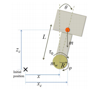
Fig. 2 Segway’s relevant parameters [15]
Where;
- \(x\) is the horizontal position of the center of the wheel.
- \(\varphi\) is the clockwise rotation angle of the wheel from the horizontal axis
- \(\theta\) is the clockwise rotation angle of the Zumo32u4 from the horizontal axis
- \(m\) is the mass of the entire robot
- \(m_w\) is the mass of the wheel
- \(R\) radius of the wheel
- \(L\) length between the center of the wheel and the COM
- \(\tau_0\) is the applied torque
- \(I\) inertia of the body part
- \(I_w\) inertia of the wheel
System’s dynamics equations
The obtained differential equations of the system in [15] are;
With,
Model Adaptation
In [15] they define \(L\) as in (3) with the variables define as in Fig. 3.
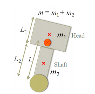
Fig. 3 Center of Mass calculation [15]
Similarly [15] defines the inertia momentum of the robot as in (4).
Given the geometry of the Zumo32u4 we consider that \(m_1 = 0\) and \(L_1 = 0\). Therefore the distance to the COM and the inertia momentum can be calculated \(L = \frac{L_2}{2}\) and \(I = \frac{1}{12}m_2L_2^2\), respectively.
Furthermore, the model in [15] consider a normal wheel. In our Zumo32u4 we have a caterpillar system. (5) shows how the inertia moment of the caterpillar system was calculated.
Where the \(I_{w_1}\) and \(I_{w_2}\) are the inertia moment of the both wheels and \(I_c\) is the inertia moment of the caterpillar band. In our case both wheels are equal and can be calculated as in (6)
Additionally the inertia of the caterpillar band can be calculated as shown in (7). Where \(m_c\) is the mass of the caterpillar band.
Finally the inertia moment of the entire caterpillar system can be calculated as in (8).
Input Adaptation
The model in [15] defines the input to be the torque \(\tau_0\). Since the actual input to our system is the PWM applied to the motors we can use the equation defined in the subsection Motors of the chapter Zumo32u4, shown in (9).
Merging (9) and (2) we obtain;
With;
State Variable Model
Finally the state variable model of the system can be calculated as shown in (10).
With the state variable vector;
And the constant matrices;
| [15] | (1, 2, 3, 4, 5, 6, 7, 8) Mie Kunio Ye Ding, Joshua Gafford. Modeling, simulation and fabrication of a balancing robot. Technical Report, Harvard University, Massachusettes Institute of Technology, 2012. |