LQR Controller Design

The controller to be implemented is a full-state feedback controller. The LQR controller was selected. Fig. 4 shows the block diagram of the entire system to be implemented.

Fig. 4 Full-state feedback block diagram

Physical parameters

All the parameters needed for the model can be seen in Listing 6

Listing 6 Physical constant script scripts/load_physical_constants.m [1]

% Sampling constants
T_s = 20e-3;
f_s = 1/T_s;

% Constants (context)
m = 0.24200; % Mass of the zumo
m_1 = 0;
m_2 = m;
L_1 = 0;
L_2 = 0.062;
L = L_2/2 + (L_1 + L_2) * m_1/(2*m); % Height of the zumo
beta_m = 0.01;
beta_gamma = 0.01;

g =  9.8100; % Gravitational constant
R = 0.019; % Wheel radius

I = m_1*(L_1/2 + L_2)^2 + (m_2*L_2^2)/12; % Inertial momentum

m_w = 0.004; % Mass of the wheel
m_c = 0.009; % Mass of the caterpillar band

I_w_i = m_w*R^2; % Inertia momentum of wheels
I_c = m_c*R^2; % Inertia momentum of Caterpillar band
I_w = 2*I_w_i + I_c; % Inertia momentum of Caterpillar system

% Motor's constants
motor_stall_torque = 0.211846554999999; % According to specs 30 oz-in
pulse2torque = motor_stall_torque/400;

Note

For \(\beta_m\) and \(\beta_\gamma\) are set to a dummy value as in [15].

Model

To setup the model the script in Listing 7 was used.

Listing 7 Get State Variable Model script scripts/get_ssmodel.m [1]

function model = get_ssmodel()

  % Consants (context)
  load_physical_constants

  E = [(I_w + (m_w + m)*R^2) m*R*L;
       m*R*L (I + m*L^2)];

  F = [(beta_gamma + beta_m) -beta_m;
       -beta_m beta_m];

  G = [0; -m*g*L];

  H_1 = [1; -1] * pulse2torque;

  states = size(E, 1);

  A = [zeros(states) eye(states);
       zeros(states, 1) -inv(E)*G -inv(E)*F];
  B = [zeros(states, 1);
       -inv(E)*H_1];
  C = [1 0 0 0;
       0 1 0 0;
       0 0 1 0;
       0 0 0 1];
  D = [0; 0; 0; 0];

  model = ss(A, B, C, D);

end

A second script, shown in Listing 8 was also added to get the model that also obtains the transfer function \(H(s) = \frac{\Theta(s)}{S(s)}\). Where, \(S(s)\) is the Laplace transform of the \(speed_{PWM}\) function. This transfer function was used to further analysis not presented in this documentation.

Listing 8 Get Model script scripts/get_model.m [1]

function [plant, model] = get_model()

  % Get the state variable model
  model = get_ssmodel();

  % Get the transfer function
  plant = tf(model);
  plant = plant(2);

end

Controllability

Before the actually designing the controller we need to check it’s controllability. The controllability check done can be seen in Listing 9.

Listing 9 Check controllability scripts/lqr_design.m [1]

% Check controlability
co =  ctrb(model);
if (rank(co) > n_states)
  disp(" -> Error! System isn't controllable");
  return;
else
  disp(" -> Great! System is controllable");
end

Observability

Similarly, the system’s observability has to be also verified. This verification is shown in Listing 10.

Listing 10 Check Observability scripts/lqr_design.m [1]

ob = obsv(model);
if (rank(ob) > n_states)
  disp(" -> Error! System isn't observable");
  return;
else
  disp(" -> Great! System is observable");
end

Control Law

To obtain the control law \(K\) the script in Listing 11.

Listing 11 Control Law Calculation scripts/lqr_design.m [1]

Q = eye(size(model.a,1));

R = 1

[K, X, P] = lqr(model, Q, R);

K_s = K*pi/180;

Note

• As in [15] equally weighted states and outputs were used. Therefore, \(Q = I\) and \(R = 1\). Where, \(I\) is an identity matrix with the size of \(A\).
• A scaled control law \(K_s\) is also calculated. The scale factor is needed because the angles measured by accelerometer/gyro and encoders was done in degrees.

The obtained control law is shown in (11). And the scaled version in (12)

(11)\[K = \begin{bmatrix} 1 & 483.6133 & 10.0038 & 20.3053 \end{bmatrix}\]

(12)\[K_s = \begin{bmatrix} 0.0175 & 8.4406 & 0.1746 & 0.3544 \end{bmatrix}\]

Controller Simulation

After designing the control law the controller is simulated as shown in Listing 12.

Listing 12 Controller simulation excerpt scripts/lqr_design.m [1]

Ac = model.a - model.b*K;
sys_cl = ss(Ac, model.b, model.c, model.d);
figure(1);
clf(1)
impulse(sys_cl);

The simulation results can be seen in Fig. 5. Since the \(\frac{d\varphi}{dt}\) and \(\frac{d\theta}{dt}\) are faster variables a zoomed result simulation result can also be seen in Fig. 6.

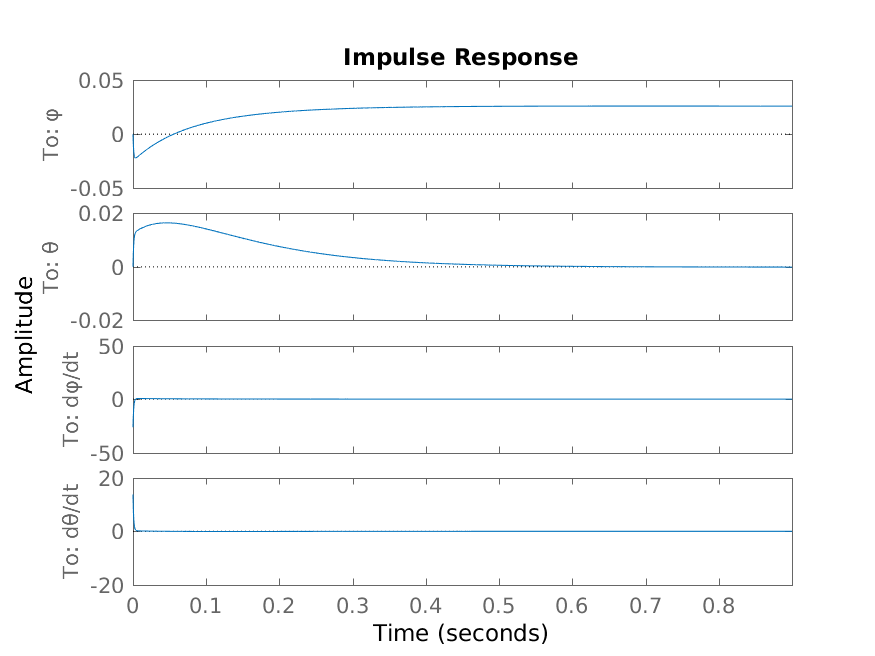
Fig. 5 LQR Design Simulation Results

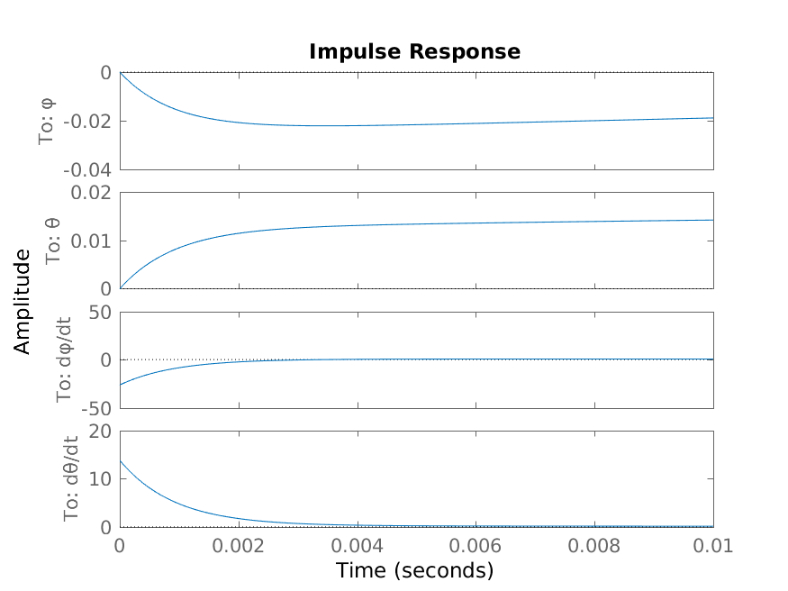
Fig. 6 LQR Design Zoomed Simulation Results

Further Features

Arduino Pretty Printing

For rapid deployment and testing the scripts/lqr_design.m also prints the scaled control law in the Arduino language. An example output can be seen in Listing 14 and the script excerpt that implement this functionality in Listing 13.

Listing 13 Arduino Code control law generator scripts/lqr_design.m [1]

disp("Control Law")
K_string = strcat("const float K[", num2str(size(model.a,1)), "] = {");
for k = 1:size(K, 2)
  if ~(k == 1)
    K_string = strcat(K_string, ", ");
  end
  K_string = strcat(K_string, num2str(K_s(k)));
end
K_string = strcat(K_string, "};");
disp("K")
disp(K_string)

Listing 14 Arduino Code control law generator output

Control Law
K
const float K[4] = {0.017453, 8.4406, 0.1746, 0.35439}

Closed-Loop Poles

scripts/lqr_design.m also print out the closed-loop poles. An example output can be seen in Listing 15.

Listing 15 Closed-loop printing output example

P =

 1.0e+03 *

 -1.0872
 -0.0000
 -0.0083
 -0.0178

Full-compensator design

In scripts/lqr_design.m the full compensator design flow is implemented but since it’s not being implements it’s was left out of this documentation.

[1]	(1, 2, 3, 4, 5, 6, 7, 8) Pedro Cuadra Meghadoot Gardi. Pjcuadra/zumogetway. August 2017. URL: https://github.com/pjcuadra/zumosegway.

[15]	(1, 2) Mie Kunio Ye Ding, Joshua Gafford. Modeling, simulation and fabrication of a balancing robot. Technical Report, Harvard University, Massachusettes Institute of Technology, 2012.